Over the past year I helped a few people pick mortgages while buying their homes by helping them visualize different mortgage options from different companies. In a seller’s market, like where I live, you only get a few days to pick from a number of different mortgages that all offer different fees, points, and interest rates that all influence the monthly rate that you pay.
Given all this data, how do you compare the difference options and decide which one to go with? The lowest monthly rate isn’t always the best option.
A brief summary of mortgages
Note this article will be focused on US mortgages in 2020. Other countries may have difference regulations, but hopefully the math should be reusable. Additionally, I am not a/your tax accountant, nor a lawyer, so this should be purely informational that you can use to reference.
When you view a mortgage offering, you’ll generally get a table of different offerings that look something like:
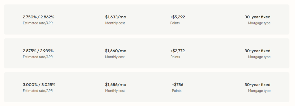
An example mortgage rate table
The estimated rate tells you the interest rate you’ll pay. The APR is the interest rate combined with the fees, but since fees are treated different than interest for tax purposes, we’ll separate them out. Points are money that you pay upfront to buy a lower interest rate. This point will visualize the differences later.
The above table hides some of the data points we care about, but in the US all mortgage providers are supposed to provide you with a loan estimate document similar to below document. The CFPB/Consumer Financial Protection Bureau has an explainer on this document.
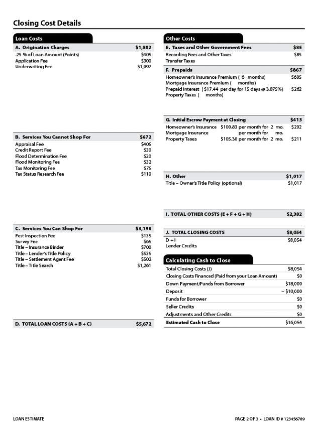
When looking at this document, we care about the origination charges. I won’t include any escrow because I always exclude escrow from mortgages.
Coding
For simplicity, I started by searching for financial related web pages explaining how to model finances using Python, Pandas, and matplotlib. I choose these tools because they were quite popular with data analytics and number crunching problems and I knew there would be libraries and examples available.
I found this blog post that I used as a baseline to start coding and created a Zeppelin notebook in my own Zeppelin instance.
First, some basic Python imports
 1
 2
 3
 4
 5
 6
 7
 8
 9
10
11
12
13
| import pandas as pd
from datetime import date
import numpy as np
from collections import OrderedDict
from dateutil.relativedelta import *
import matplotlib.pyplot as plt
from IPython.core.pylabtools import figsize
plt.style.use('ggplot')
import matplotlib.ticker as ticker
money_formatter = ticker.FormatStrFormatter('$%1.0f')
|
Next, we need to define an amortization table function. Given the inputs, these functions will return a Pandas DataFrame that contains a monthly breakdown of the different payments and costs that we’ll build upon.
Inputs:
amortization_table
| Parameter Name | Example | Description |
| principal | 500000 | Amount of money for the loan (total house - down payment) |
| interest_rate | 0.03 | 0-1 representing the interest rate APY |
| years | 30 | Number of years (e.g. 15 or 30) |
| addl_principal | | |
| annual_payments | 12 | Number of payments per year (usually 12) |
| start_date | date(2022, 1, 1) | Represents the date when the loan will start. e.g (date.today()) |
| fees | 999 | Origination fees |
| points | 1000 | |
 1
 2
 3
 4
 5
 6
 7
 8
 9
10
11
12
13
14
15
16
17
18
19
20
21
22
23
24
25
26
27
28
29
30
31
32
33
34
35
36
37
38
39
40
41
42
43
44
45
46
47
48
49
50
51
52
53
54
55
56
57
58
59
60
61
62
63
64
65
66
67
68
69
70
71
72
73
74
75
76
77
78
79
80
81
82
83
84
85
86
87
88
89
90
91
92
93
94
95
96
97
| # Original credit: https://pbpython.com/amortization-model-revised.html
def amortize(principal, interest_rate, years, pmt, addl_principal=0, start_date=date.today(), annual_payments=12):
"""
Calculate the amortization schedule given the loan details.
:param principal: Amount borrowed
:param interest_rate: The annual interest rate for this loan
:param years: Number of years for the loan
:param pmt: Payment amount per period
:param addl_principal: Additional payments to be made each period.
:param start_date: Start date for the loan.
:param annual_payments: Number of payments in a year.
:return:
schedule: Amortization schedule as an Ordered Dictionary
"""
# initialize the variables to keep track of the periods and running balances
p = 1
beg_balance = principal
end_balance = principal
while end_balance > 0:
# Recalculate the interest based on the current balance
interest = round(((interest_rate/annual_payments) * beg_balance), 2)
# Determine payment based on whether or not this period will pay off the loan
pmt = min(pmt, beg_balance + interest)
principal = pmt - interest
# Ensure additional payment gets adjusted if the loan is being paid off
addl_principal = min(addl_principal, beg_balance - principal)
end_balance = beg_balance - (principal + addl_principal)
yield OrderedDict([('Month',start_date),
('Period', p),
('Begin Balance', beg_balance),
('Payment', pmt),
('Principal', principal),
('Interest', interest),
('Additional_Payment', addl_principal),
('End Balance', end_balance)])
# Increment the counter, balance and date
p += 1
start_date += relativedelta(months=1)
beg_balance = end_balance
def monthly_payment(principal, years, interest_rate, annual_payments=12):
return -round(np.pmt(interest_rate / annual_payments, years * annual_payments, principal), 2)
def amortization_table(principal, interest_rate, years,
addl_principal=0, annual_payments=12, start_date=date.today(), fees=0, points=0):
"""
Calculate the amortization schedule given the loan details as well as summary stats for the loan
:param principal: Amount borrowed
:param interest_rate: The annual interest rate for this loan
:param years: Number of years for the loan
:param annual_payments (optional): Number of payments in a year. Default 12.
:param addl_principal (optional): Additional payments to be made each period. Default 0.
:param start_date (optional): Start date. Default first of next month if none provided
:return:
schedule: Amortization schedule as a pandas dataframe
summary: Pandas dataframe that summarizes the payoff information
"""
# Payment stays constant based on the original terms of the loan
payment = monthly_payment(principal, years, interest_rate, annual_payments)
# Generate the schedule and order the resulting columns for convenience
schedule = pd.DataFrame(amortize(principal, interest_rate, years, payment,
addl_principal, start_date, annual_payments))
schedule = schedule[["Period", "Month", "Begin Balance", "Payment", "Interest",
"Principal", "Additional_Payment", "End Balance"]]
# Convert to a datetime object to make subsequent calcs easier
schedule["Month"] = pd.to_datetime(schedule["Month"])
schedule["Payment"].iloc[0] += points + fees
schedule["Interest"].iloc[0] += points
schedule["Total Payment"] = schedule["Payment"] + schedule["Additional_Payment"]
#schedule["Total Payment"].iloc[0] += fees
#Create a summary statistics table
payoff_date = schedule["Month"].iloc[-1]
stats = pd.Series([payoff_date, schedule["Period"].count(), interest_rate,
years, principal, payment, addl_principal,
schedule["Interest"].sum()],
index=["Payoff Date", "Num Payments", "Interest Rate", "Years", "Principal",
"Payment", "Additional Payment", "Total Interest"])
schedule.set_index('Month', inplace=True, drop=False)
return schedule, stats
|
With these functions, I can now create different visualizations.
Let’s plot a per month how much I’m paying for interest vs principal.
 1
 2
 3
 4
 5
 6
 7
 8
 9
10
11
12
13
| home_value = 500000
down_payment = 0.2
interest = 0.03
fig, ax = plt.subplots()
ax.yaxis.set_major_formatter(money_formatter)
mortgage = amortization_table(home_value * (1 - down_payment), interest, 30)[0]
ax.plot(mortgage[['Principal', 'Interest']])
ax.yaxis.set_major_formatter(money_formatter)
ax.legend(['Principal', 'Interest'])
ax.title.set_text("Amortization Table")
|
Running that gives a graph like below. In the beginning, I’m paying mostly towards interest vs principal. Classic banks.
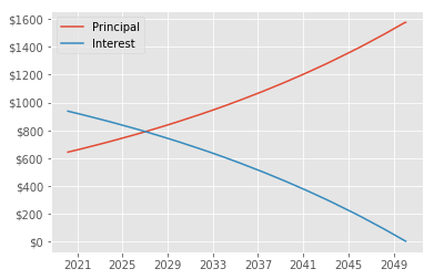
An amortization table showing monthly payments towards interest or principal.
Let’s try playing around with different payment scenarios. How does making extra payments affect the pay-off?
 1
 2
 3
 4
 5
 6
 7
 8
 9
10
11
12
13
14
15
16
17
18
19
20
| payment_table = []
home_value = 500000
down_payment = 0.20
interest = 0.03
for extra_pay in range(0, 1000, 100):
mortgage = amortization_table(home_value * (1 - down_payment), interest, 30, addl_principal=extra_pay, start_date=date(2020, 3, 1))
mortgage[0]['Extra Payment'] = extra_pay
payment_table.append(mortgage[0])
amounts = []
fig, ax = plt.subplots()
ax.yaxis.set_major_formatter(money_formatter)
for type in payment_table:
amounts.append("+$%s/mo" % type['Extra Payment'][0])
ax.plot(type['Month'], type['End Balance'])
ax.title.set_text("Extra payments pay balance faster")
ax.legend(amounts)
|
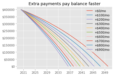
Clearly paying more money per month causes you to pay a mortgage faster, but let’s expand this to introduce the concept of opportunity cost.
Opportunity Cost
Opportunity cost is an economic concept that considers not just the cost of a good or service, but what is the cost that you lose out on by deciding not to buy an alternative good or service. For example, instead of spending $100 today on a good, you could invest it something that yields 5% real (inflation adjusted) and have $105 in one year. Your opportunity cost of that good is $105. The same concept can be applied to mortgages.
A mortgage is usually a fixed rate over large number of years. At the time of this writing, they were about 3% for 30 years. If you put an additional $100 into the mortgage as an extra principal payment, yes that reduces your principal and interest paid by some small amount, but you earn a guaranteed 3%, no more, no less than that for that $100. Compared to checking and saving accounts at a paltry 0.1% - 0.5% interest rate, this is clearly better. But compared to the stock market which has returned an average of 10% per year, this is lower.
However, it’s important to note that you must compare the return rate combined with the risk of that investment. A stock can return -10% or +30% and still average to be +10% whereas a mortgage will always return the interest rate.
To calculate the opportunity cost of an additional payment, I’m going to assume that an individual will either pay into the mortgage or put the money into a stock market yield 8% (I’ll chart different returns later.) I’m also going to adjust for the tax deduction of the interest payments.
First, some simple utility code. Define the standard deduction which is $12,500 for 2020 and a function to normalize everything to 30 years (in case of comparing a 15 year to a 30 year mortgage).
1
2
3
4
5
6
7
| standard_deduction = 12500 # US Single Deduction 2020
def extend_to_max(start_date, table):
thirty_years = pd.date_range(start=start_date, periods=(30 * 12), freq='MS', closed='left')
table = table.reindex(thirty_years)
table['Month'] = thirty_years
return table.fillna(0)
|
Next, another utility function that takes a Pandas Series stating how much money to put into the market per month, and returns a Series stating the value of the stock at the end of each month. This is useful to calculate the growth over time and allows me to define separate investment amounts depending on the month; for example, the first month has origination fees that don’t appear in later months.
 1
 2
 3
 4
 5
 6
 7
 8
 9
10
| def calculate_stock_value(investment, returns):
output = []
prev = 0
for tick in investment:
value = tick + (prev * (1 + (returns / 12)))
output.append(value)
prev = value
previous_gains = pd.Series(output, index=investment.index)
return investment + previous_gains # The value of the money combined with the additional money that we added this month
|
Next, the meat of this equation. First calculate the $ amount of deductions (property taxes + interest payments) adjusted by the tax bracket. Since these are deductible, we assume that we’ll get this extra month per month to invest.
Then we can calculate how much each month we have to invest. total_bucket defines a set amount of money that could go either to stocks or to the mortgage. Out of the total bucket, we must pull out the monthly payment, then we adjust for the tax deduction, which gives some money back. That gives an equation like $3k - Principal - Interest + TaxDeduction(interest) * TaxBracket) = Remaining.
The Remaining (in the investment variable) is compounded monthly based on the expected returns. The equity in the house (i.e. how much of the house you own) is the cumulative sum of the principal payments. That gives us a per-month net value calculation stating how much these two assets are theoretically worth.
 1
 2
 3
 4
 5
 6
 7
 8
 9
10
11
| tax_bracket = 0.32
def adjusted_networth(total_bucket, table, max_payment, property_taxes, returns, initial_invest = 0):
table['Tax Deduction'] = (table['Interest'].clip(lower=0) + (property_taxes / 12) - (standard_deduction / 12)) * (tax_bracket)
table['AfterTaxes'] = table['Total Payment'] - table['Tax Deduction']
table['Investment'] = investment = (total_bucket - table['AfterTaxes']).clip(lower=0) # Extra money available for mortgage or investment
table['Investment'].iloc[0] += initial_invest
table['StockValue'] = calculate_stock_value(investment, returns) # The value of the money combined with the additional money that we added this month
return table['StockValue'] + table['Equity'] # Equity in house combined with value of investment
|
Let’s plot it out:
 1
 2
 3
 4
 5
 6
 7
 8
 9
10
11
12
13
14
15
16
17
| loan_value = 500000
monthly_total_bucket = 4000
yr_property_taxes = 5000
expected_mkt_returns = 0.08
amounts = []
fig, ax = plt.subplots()
for extra_pay in range(0, 1500, 200):
mortgage, stats = amortization_table(loan_value, 0.03, 30, addl_principal=extra_pay, start_date=date.today())
amounts.append("+$%s/mo" % extra_pay)
mortgage = extend_to_max(date.today(), mortgage)
mortgage['NetWorth'] = adjusted_networth(monthly_total_bucket, mortgage, yr_property_taxes, expected_mkt_returns)
ax.plot(mortgage['Month'], mortgage['NetWorth'])
ax.yaxis.set_major_formatter(money_formatter)
ax.title.set_text("Net worth")
ax.legend(amounts)
|
Running that gives us the following plot. So assuming, the market returns 8% on average, doing just the minimum payments and investing it elsewhere will theoretically give the best returns at the current mortgage interest rates.
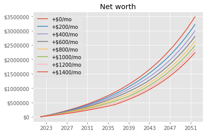
Of course, past performance of the stock market does not mean that it will continue to yield that and personal risk tolerances and goals may lead you to make different choices.
Comparing Mortgage Options
Now with some simple basics down, let’s compare a number of different loan options. First, let’s get all input parameters inputted. The different mortgages come from the different offerings that they all provide. Below is some sample interest rates with different years
 1
 2
 3
 4
 5
 6
 7
 8
 9
10
11
| # Multiple loan products
property_taxes = 5000
start_date = date(2021, 11, 1)
home_value = 500000
total_bucket = 4000
mortgages = [
{"down_pct": 0.25, "company": "A", "rate": 0.0225, "fees": 614, "years": 30, "points": 11081 },
{"down_pct": 0.25, "company": "A", "rate": 0.0275, "fees": 614, "years": 30, "points": -3609 },
{"down_pct": 0.2, "company": "A", "rate": 0.02, "fees": 614, "years": 15, "points": 0 },
]
|
Then with that data, iterate over all combinations of mortgages along with different stock market values
 1
 2
 3
 4
 5
 6
 7
 8
 9
10
11
12
13
14
15
16
17
18
19
20
21
22
23
24
25
26
27
28
| output = []
#fig, ax = plt.subplots()
opportunity_return_options = np.arange(0.00, .15, 0.05) # Range of returns the stock market *could* give
fig, subplots = plt.subplots(len(opportunity_return_options), 1, sharex=True, sharey=True, figsize=(10, 10))
legends = []
max_rate = max(mortgages, key = lambda x: x["points"])["rate"]
total_bucket = monthly_payment(home_value * (1 - 0.25), 30, max_rate)
for (stonk_market_returns, subplot) in zip(opportunity_return_options, subplots):
mortgage_labels = []
subplot.title.set_text("If the stock market returns %s%%" % (stonk_market_returns * 100))
subplot.yaxis.set_major_formatter(money_formatter)
for extra_payment in [0]:
for product in mortgages:
loan_principal = home_value * (1 - product["down_pct"])
payment = monthly_payment(loan_principal, product["years"], product["rate"])
table = amortization_table(loan_principal, product["rate"], product["years"], addl_principal=extra_payment, start_date=start_date, fees=product["fees"], points=product["points"])[0]
table = extend_to_max(start_date, table)
table["Equity"] = table["Principal"].cumsum() + (home_value * product["down_pct"])
table['TotalWorth'] = adjusted_networth(total_bucket, table, property_taxes, stonk_market_returns) # Equity in house combined with value of investment
time = table #table[table['Month'] < '2026-02-01']
avg_invest = time['Investment'].mean()
rate = product["rate"] * 100
mortgage_labels.append("%s %s%% for %d yrs final=$%d" % (product["company"], rate, product["years"], time['TotalWorth'].max()))
subplot.plot(time['Month'], time['TotalWorth'])
subplot.legend(mortgage_labels)
|
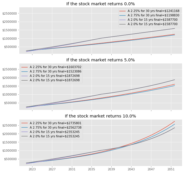
That gives us a chart like below showing the relationship between the stock market returns, along with my net worth (purely example values.)
This is just the start what you can do when you model your finances in Pandas. Since it’s all in code, I can make it more advanced than simple web calculators that aren’t able to account for tax differences or opportunity costs. I even extended this to visualize a refinancing a mortgage.